(19) 變分 Hamiltonian vs Lagrangian

前面簡述完Hamiltonian和Lagrangian，乍看之下會覺得$H$比$L$多了一個自由度$(p,q)$，我們下面用簡單的等加速運動例子和角動量守恆來看待這件事情。

比較一：加速

Lagrangian

牛頓力學和$L$的EOM告訴我們

\[\frac{d^2 x}{dt^2}=a=\text{some constant}\]

真實軌跡的解是

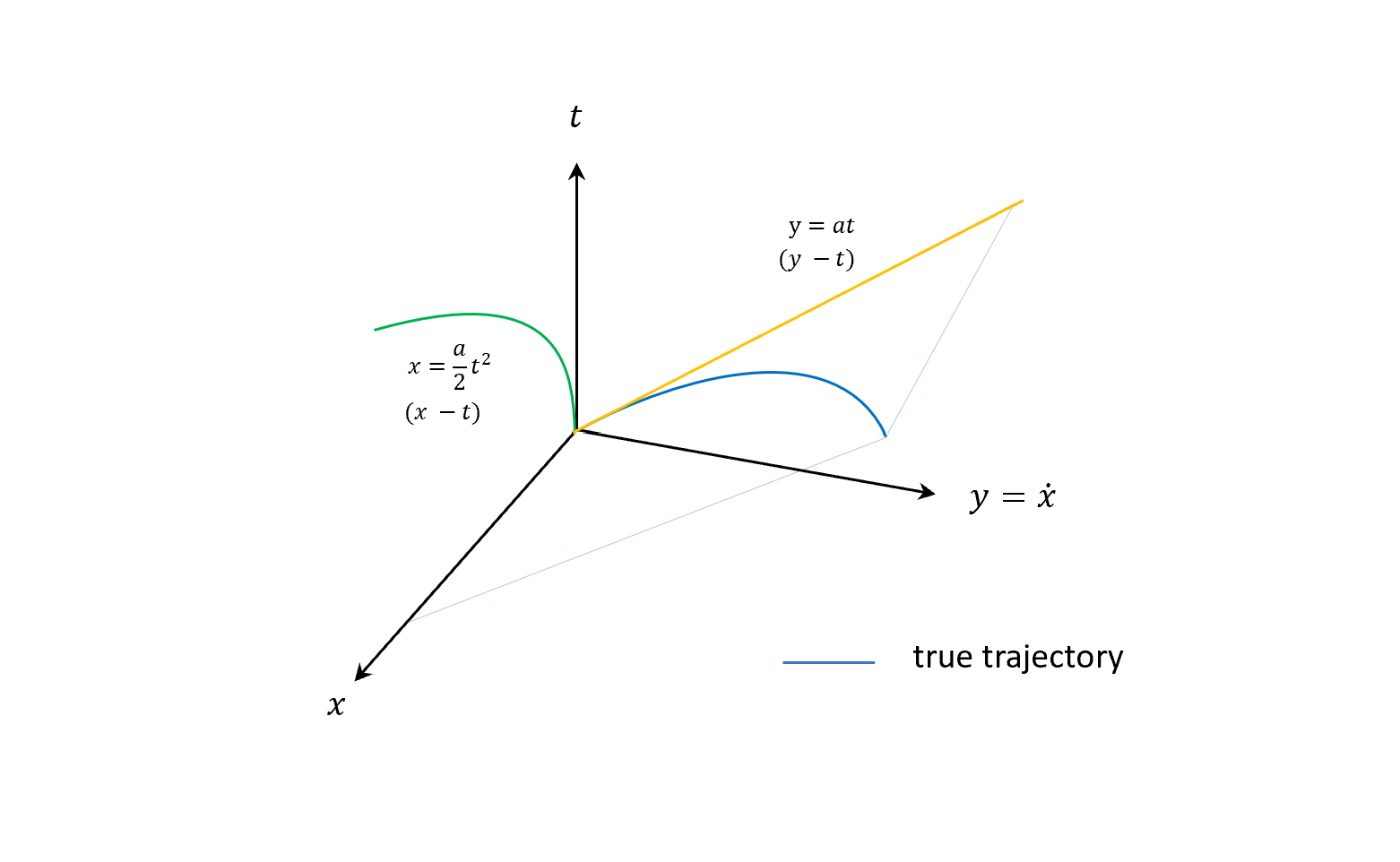
\[\left\{ \begin{array}{ll} x(t)=\frac{a}{2}t^2\\ \dot{x}(t)=at \end{array} \right.\]

現在令

\[y=\dot{x}\]

把解畫在$x-y-t$上面，可以得到$x-t$是拋物線，$y-t$是直線，然後顯示到3-D空間的話，true trajectory會是藍色那條。

現在加一點variation，$\epsilon$是微小的正數，灰色就是variation的軌跡

\[\left\{ \begin{array}{ll} x(t)\equiv x^*(t)+\epsilon\sin\frac{2\pi t}{T}\\ \dot{x}(t)=\dot{x^*}(t)+\epsilon 2\pi \cos\frac{2\pi t}{T} \end{array} \right.\]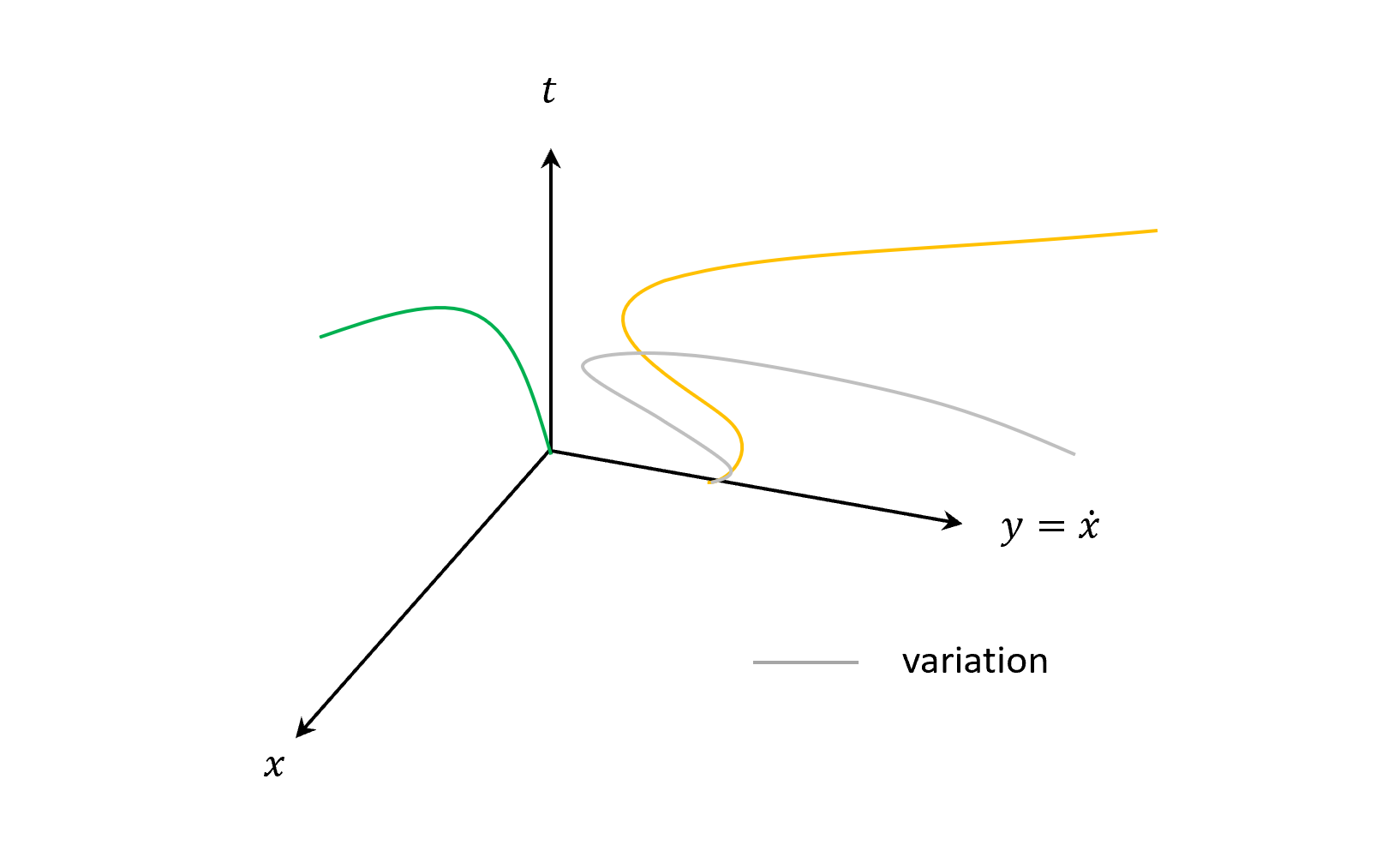

簡而言之

\[x(t)\equiv x^*(t)+\delta x(t)\\ y(t)\equiv y^*(t)+\delta y(t)\\ \delta (\text{something})=\text{small variation at something}\]

注意其中

\[\delta y=\diff{\delta x}{t}\]

是我們自己強制定義的，所以若我們決定綠線$x(t)$，橘線$y(t)$就已經被限制住(無自由度)，這裡的$\delta y$和$\delta x$的關係緊密。

最後得varitaional principle within the Lagrangian formulation:

若

\[(x(t),y(t))=\left(x^*(t),\diff{x^*(t)}{t}\right)\]

是真實軌跡，則

\[\int_{0}^{T} L(x(t),y(t),t)\, dt\]

就會是極值。而其中一個自由度的限制是

\[y=\diff{x}{t}\]

Hamiltonian

現在換到Hamiltonian，我們改寫EOM，並且先當作數學問題，多個未知的$p$

\[\left\{ \begin{array}{ll} \diff{x}{t}=p\\ \diff{p}{t}=a \end{array} \right.\]

真實軌跡

\[\left\{ \begin{array}{ll} x(t)=\frac{a}{2}t^2\\ p=at \end{array} \right.\]

畫出來的圖會和前面一樣

現在加variation

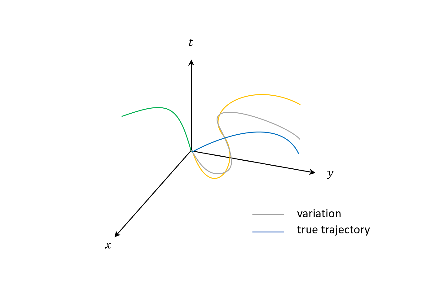
\[\left\{ \begin{array}{ll} x(t)\equiv x^*(t)+\epsilon\sin\frac{2\pi t}{T}\\ y(t)=y^*(t)+\delta p(t) \end{array} \right.\]

注意這時$\delta p(t)=\delta y$可以是”任意”的小函數，所以原本的綠色線照畫，橘色線不再特定，只要畫過去的3D線可以再投影到綠線就可以了。

最後得varitaional principle within the Hamiltoian formulation:

若

\[(x(t),y(t))=(x^*(t),p^*(t))\]

是真實軌跡，則

\[\int_{0}^{T} p(t)\,dx-H(x,p,t)\, dt\]

就會是極值。而我們發現

\[p^*(t)=\diff{x^*}{t}\]

完全是後見之明。

所以雖然Hamiltonian的自由度更大，想怎麼vary隨便你，但取極值後的true trajectory(真正關心的)和Lagrangian相同！從這點來看的話，Hamiltonian和Lagrangian兩者其實沒有差。

比較二：角動量守恆

從自由度和變分的角度出發，我們知道最基本的變分，就是把真實軌跡拿來當參考值，然後作任意小改變，來得知系統隨時間怎麼變化，然後掌握系統的所有事情。

但其實沒有告訴你一定要考慮所有可能的變化，若只是單純討論某一類特殊的變化，即便僅是得知系統部分的資訊，即便不能知道整個系統動態隨時間的變化，也已經夠了。

現在我們就來看角動量守恆，這個在之前的第十一節和第十二節都有用Lagrangian算過，現在用Hamiltonian來證。

一樣$H$隨著$q,p$的改變，但這個改變我們設只跟$q,p$的長度有關。

(這樣的假設像是討論向心力場這類的問題就可以用，因為動能是$p^2$，位能與中心的距離有關。)

因此我們定 Hamiltonion for a particle is of form：

\[H(\|\vv{q}\|,\|\vv{p}\|)\]

加上對著$\hat{n}$軸做旋轉的擾動變量

\[\vv{q}=\vv{q}^*+\epsilon\hat{n}\times\vv{q}^*\\ \vv{p}=\vv{p}^*+\epsilon\hat{n}\times\vv{p}^*\\ \hat{n}: \text{some constant unit vector}\\ \epsilon: \text{arbitraty but small}\]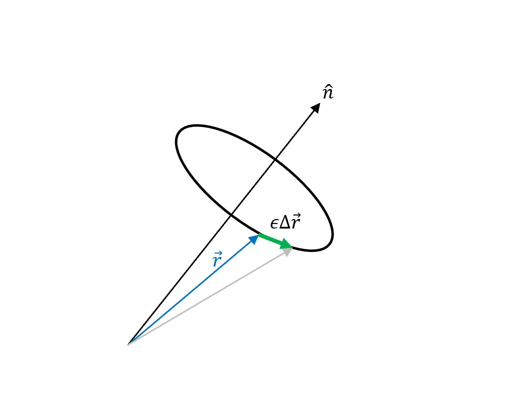

其中$q,p$的擾動量只在$t_1, t_2$間有，表示真實軌跡走一走到某個時間點做改變，在某個時間之後再變回真實軌跡。

\[\left\{ \begin{array}{ll} \theta(t-t_1)-\theta(t-t_2)\\ \theta(t-t_1)-\theta(t-t_2) \end{array} \right.\] \[\theta: \text{heaviside function}\]

先算$H$的變分

\[\delta{H}=H(\|\vv{q}\|,\|\vv{p}\|)-H(\|\vv{q}^*\|,\|\vv{p}^*\|)=0\]

若只算到$\mathcal{O}(\epsilon)$，那就會是0。

因為

\[\|\vv{r}\|=\|\vv{r}^*+\epsilon\hat{n}\times\vv{r}^*\|\\\]

算長度時因為

\[\vv{r}\perp\hat{n}\times\vv{r}\]

所以取平方時，兩個內積為0，只會剩下${\vv{r}^* }^2+\epsilon^2(\hat{n}\times\vv{r}^*)^2 $，差別是二階$\epsilon$。

在這裡我們只看一階，$\delta{H}=0$

接著來算變分公式

\[\begin{align*} 0&=\delta\left(\int{\vv{p}\cdot d\vv{q}-Hdt}\right)\\ &=\int\delta\vv{p}\cdot d\vv{q}^*+\vv{p}^*\cdot d(\delta\vv{q})-\delta Hdt\\ &=\int\delta\vv{p}\cdot d\vv{q}^*+\vv{p}^*\cdot d(\delta\vv{q})\\ &=\epsilon\int_{t=0}^{t=T}\hat{n}\times\vv{p}^*\left(\theta(t-t_1)-\theta(t-t_2)\right)\cdot d\vv{q}^*+\epsilon\int_{t=0}^{t=T}\vv{p}^*\cdot d\left(\hat{n}\times\vv{q}^*\left(\theta(t-t_1)-\theta(t-t_2)\right)\right)\\ &\quad(\because \text{只有$t_1, t_2$有變化})\\ &=\epsilon\int_{t_1}^{t_2}(\hat{n}\times\vv{p}^*)\cdot d\vv{q}^*\\ &\quad+\epsilon\int_{t=0}^{t=T}\vv{p}^*\cdot\left(\hat{n}\times d\vv{q}^*\right)\left(\theta(t-t_1)-\theta(t-t_2)\right)\\ &\quad+\epsilon\int_{t=0}^{t=T}\vv{p}^*\cdot\left(\hat{n}\times\vv{q}^*\right)\left(\frac{d}{dt}\left(\theta(t-t_1)-\theta(t-t_2)\right)\right)dt\\ &=\epsilon\int_{t_1}^{t_2}(\hat{n}\times\vv{p}^*)\cdot d\vv{q}^*+\epsilon\int_{t_1}^{t_2}\vv{p}^*\cdot(\hat{n}\times d\vv{q}^*)+\epsilon\int_{t=0}^{t=T}\vv{p}^*\cdot\left(\hat{n}\times\vv{q}^*\right)\left(\delta(t-t_1)-\delta(t-t_2)\right)dt\\ &\quad(\because\vv{p}^*\cdot\left(\hat{n}\times d\vv{q}^*\right)=d\vv{q}^*\cdot\left(\vv{p}^*\times\hat{n}\right))\text{ 第一項和第二項相消}\\ &=\epsilon\vv{p}^*\cdot\left(\hat{n}\times \vv{q}^*\right)\bigg |_{t=t_2}^{t=t_1}=0\\ &\quad(\because\text{積分後是}\int_{0}^{t_1}-\int_{0}^{t_2}\text{，所以上下限剛好顛倒}) \end{align*}\]

因此得

\[\hat{n}\cdot\left(\vv{q}^*\times\vv{p}^*\right)\bigg |_{t=t_2}= \hat{n}\cdot\left(\vv{q}^*\times\vv{p}^*\right)\bigg |_{t=t_1}\]

把$q$想成長度，$p$是動量，則此式得證角動量守恆。

可以和之前用Lagragian推導做比較，$L$是$q$變化，$\dot{q}$就會被決定下來；$H$是$q,p$都可自由被決定的，但我們可以只關注部分的變動量，得到系統的部分資訊，也能得到有意義且一樣的結果。

總結比較

Item	Lagrangian	Hamiltonian
Transformation	From $L$ to $H$: Given $L(q,q’,t) \quad(q’$ 先當作純數學的變數) Define $p\equiv\pdv{L(q,q’,t)}{q’}$ So can express $q’\equiv q’(q,p,t)$ Next define $H(q,p,t) = pq’(q,p,t)-L(q,q’(q,p,t),t)$	From $H$ to $L$: Given $H(q,p,t)$ Define $q’\equiv\pdv{H(q,p,t)}{p}$ So can express $p=p(q,q’,t)$ Next define $L(q,q’,t)=p(q,q’,t)q’-H(q,p(q,q’,t),t)$
Formula	設 $q’(t) \rightarrow \dot{q}(t)$ and consider $I_L \equiv \int_0^T L\left(q, q’ = \frac{dq}{dt}, t\right) \, dt$	Consider $I_H \equiv \int_0^T pdq - H(q, p, t) \, dt $
DOF	$ q(t) $	$q(t), p(t)$ essentially arbitrary
B.C.	$q(0) = q^* (0), q(T) = q^* (T)$	$ q(0) = q^* (0), q(T) = q^*(T) $
Claim	$ q^*(t) $ extremizes $ I_L $	$(q^* (t), p^ *(t)) $ extremized $ I_H $
Note	One can prove that $ I_L $ is minimized by $ q^*(t) $ under certain conditions such as in the case when $ T $ is small (真實軌跡會是$ I_L $取最小值，也因為自由度比較小，所以若專注在shape trajectory，會比較快找到路走)	$ I_H $ is only extremized by $ (q^* (t), p^* (t)) $ only. That is, one cannot talk about the minimization of it. (真實軌跡只能說 $ I_H $ 取極值，但因為本來就有較高的自由度去做variation，所以付出的代價就是不一定是最小值)

最後是兩者Common的性質：

若我們只考慮真實軌跡，則

\[I_L[q^*(t)] = I_H[(q^*(t), p^*(t))]\]

Prf:

\[\begin{align*} p^* dq^* - H^* dt &= \left( p^* \frac{dq^*}{dt} - H^* \right) dt \\ &= \left( p^* \frac{dq^*}{dt} - (p^* \dot{q}^* - L(q, \dot{q}, t)) \right) dt \\ &= L dt \end{align*}\]

這邊對關於Lagrangian和Hamiltonian的轉換，教科書中常見是用Legendre transformation，但對我現在的理解來說，其實就是降階和做變數變換，以下節錄一段Goldstein的文字

From the mathematical viewpoint, it can however be claimed that the $q$’s and $\dot{q}$’s have been treated as distinct variables. In Lagrange’s equations $\frac{d}{dt}\left(\frac{\partial L}{\partial \dot{q}_i}\right)-\frac{\partial L}{\partial q_i}$, the partial derivative of $L$ with respect to $q_i$ means a derivative taken with all other $q$’s and all $\dot{q}$’s constant. Similarly, in the partial derivatives with respect to $\dot{q}$, the $q$’s are kept constant. Treated strictly as a mathematical problem, the transition from Lagrangian to Hamiltonian formulation corresponds to changing the variables in our mechanical functions from $(q, \dot{q},t)$ to $(q, p,t)$, where $p$ is related to $q$ and $\dot{q}$ by $p_i=\frac{\partial L(q_j, \dot{q}_j, t)}{\partial \dot{q}_i}$. The procedure for switching variables in this manner is provided by the Legendre transformation, which is tailored for just this type of change of variable.

─ (Goldstein, H.), Classical mechanics. Pearson Education India, 3rd edn, (p.334).

$L$ & $H$ 公式例子

例子一：傳統力學

假設 Lagrangian 為

\[L=\sum_{j}\frac{m}{2}\dot{\vv{r_j}}^2-V(\vec{r})\]

其中$j$是partical index，而

\[\vec{r}\equiv(\vec{r_1}, \vec{r_2},\cdots)\]

現在改寫成矩陣的形式

\[L = \frac{1}{2}\dot{\vv{r}}^t\cdot\hat{M_0}\cdot\dot{\vv{r}}-V(\vec{r})\\ \hat{M_0}= \begin{pmatrix} m_1 & 0 & 0 & 0\\ 0 & m_2 & 0 & 0\\ 0 & 0 & \ddots & 0\\ 0 & 0 & 0 & m_j \end{pmatrix}\]

接著定義

\[\begin{align*} \vec{q}\equiv\vec{f}^{-1}(\vec{r})&\Rightarrow\vec{r}=\vec{f}(\vec{q})\\ \hat{R}\equiv\pdv{\vec{f}}{\vec{q}}&\Rightarrow\dot{\vv{r}}=\pdv{\vec{f}}{\vv{q}}\cdot\dot{\vv{q}}=\hat{R}\cdot\dot{\vv{q}} \end{align*}\]

來描述motion，所以

\[\begin{align*} L &= \frac{1}{2}\dot{\vv{r}}^t\cdot\hat{M_0}\cdot\dot{\vv{r}}-V(\vec{r})\\ & = \frac{1}{2}\left(\hat{R}\dot{q}\right)^t\cdot\hat{M_0}\cdot\left(\hat{R}\dot{\vv{q}}\right)-V\left(\vv{f}(\vv{q})\right)\\ &=\frac{1}{2}\dot{\vv{q}}^t{\hat{R}}^t\hat{M_0}\hat{R}\dot{\vv{q}}-V\\ &\equiv\frac{1}{2}\dot{\vv{q}}^t\hat{M_1}\dot{\vv{q}}-V \end{align*}\]

其中$V$被視為$\vec{q}$的函數，$\hat{M_1}$則是symmetrix “effective” mass matrix (不一定有m的因次)。

代回Hamiltonian，知

\[\vv{p}\equiv\pdv{L}{\dot{\vv{q}}}=\hat{M_1}\cdot\dot{\vv{q}}\\ \dot{\vv{q}}=\frac{1}{\hat{M_1}}\vv{p}\]

則

\[\begin{align*} H&\equiv\vv{p}^t\cdot\dot{\vv{q}}-L\\ &=\vv{p}^t\cdot\frac{1}{\hat{M_1}}\vv{p}-\frac{1}{2}\vv{p}^t\frac{1}{\hat{M_1}}\hat{M_1}\frac{1}{\hat{M_1}}\vv{p}+V\\ &=\frac{1}{2}{\vv{p}}^t\cdot\frac{1}{\hat{M_1}}\cdot\vv{p}+V\\ &=\color{red}{\left(\frac{p^2}{2m}+V\right)} \end{align*}\]

(就是總能量(動能+位能)，並且這個其實也可以對應之後讀量力薛丁格方程求穩態的Time-independent function的Hamiltonian Operator表示了)

例子二：加入電場

\[L = \frac{m}{2}\dot{\vv{q}}^2-e\phi+e\dot{\vv{q}}\cdot\vv{A}\]

其中

\[\vv{q} \text{: 3D cartesion coordinate}\\ \phi \text{: scalar potential}\\ \vv{A} \text{: vector potential}\\ e \text{: charge of the partical}\]

canonical momentum conjugate to $\vv{q}$ is

\[\vv{p}\equiv\pdv{L}{\dot{\vv{q}}}=m\dot{\vv{q}}+e\vv{A}\\ \dot{\vv{q}}=\frac{\vv{p}-e\vv{A}}{m}\]

注意這裡可以看到$\vec{p}$不再是mechanical momentum $m\dot{\vec{q}}$！

一樣來算Hamiltonian

\[\begin{align*} H&=\vv{p}\dot{\vv{q}}-L\\ &=\vv{p}\cdot\left(\frac{\vv{p}-e\vv{A}}{m}\right)-\left(\frac{m}{2}\left({\frac{\vv{p}-e\vv{A}}{m}}\right)^2-e\phi+e\frac{\vv{p}-e\vv{A}}{m}\cdot\vv{A}\right)\\ &=\frac{(\vv{p}-e\vv{A})^2}{m}-\frac{m}{2}\left(\frac{\vv{p}-e\vv{A}}{m}\right)^2+e\phi\\ &=\frac{(\vv{p}-e\vv{A})^2}{2m}+e\phi \end{align*}\]